
Geotechnical engineering libraryContact
 benesch
Formerly Geo Rail Chapter 17 — Railway Geo-Hazard Risk Management
Primary Source: Geotechnology for Railroaders Program, Module 1 — Risk Management of Railway Geo-Hazards; Keegan, T., Abbott, B. & Ruel, M., A Risk Management Framework for Ground Hazards Along Canadian National Railways; CAN/CSA-Q850-97, Risk Management: Guideline for Decision-Makers.
Apps on dirtbert.com that support this chapter. Each one runs in a web browser on a desktop or a phone, with nothing to install. How to use the apps (I.3). Tools marked TOOLS open in the Geotechnical Analysis Suite (Benesch sign-in); the orange card below lists each one by section.
NANCY pages ask you to accept the Use and Disclaimers once in each browser. MINA is a monitoring aid and is not for operational dispatch decisions.
Calculators and workbook tools from the Benesch Geotechnical Analysis Suite that support this chapter: 0 interactive calculators and 3 workbook guides. Each one is also placed inside the section it supports, in an orange tools strip.
| PM | RR Project ChecklistUsed in 1.10 Grade & Slope Stabilization Program — Roles and Process | guide only | Guide |
| PM | RR Bridge Site Recon ChecklistUsed in 1.10 Grade & Slope Stabilization Program — Roles and Process | guide only | Guide |
| PM | RR Summary of FindingsUsed in 1.13 Practical Recommendations | guide only | Guide |
Tools open on dirtbert.com and need the Benesch sign-in. Drafts pending Benesch final review, not for use in design.
Railroad track is more exposed to ground hazards than almost any other transportation corridor. Alignments driven to minimize gradient and curvature are forced across geomorphically active terrain, and the ground beneath a railroad is never static — slopes fail, rivers migrate, ballast degrades, and foundations weaken with water while trains keep getting heavier and climate extremes trigger more frequent events. This chapter establishes a systematic Risk Management (R.M.) framework for the landslide, hydraulic, and subsidence hazards that threaten track foundations, synthesizing the case-history-driven training approach used across Class I railroads with the formal risk-management methodology published by Canadian National Railway under the CAN/CSA-Q850-97 standard.
The chapter is organized around a single governing idea: Risk = Hazard × Consequence & Vulnerability. Every decision about whether a train can safely run over a section of track affected by a geo-hazard traces back to this equation, and every mitigation dollar spent should trace back to a documented, communicated risk-management process — not a reactive scramble after an incident. In the international disaster-risk vocabulary of the UN Office for Disaster Risk Reduction (UNDRR), the same idea is written Risk = Hazard × Exposure × Vulnerability: a ground hazard becomes a loss only where track, trains and people are exposed to it and vulnerable to it, and a railroad’s capacity to detect, warn and respond reduces that risk (§1.2). Key outputs of this chapter are: the three-category hazard classification system (Landslide, Hydraulic Erosion, Subsidence) used to inventory and prioritize sites; the cyclical R.M. process (Initiation → Preliminary Analysis → Risk Estimation → Risk Evaluation → Risk Control → Action/Monitoring, with Risk Communication running throughout); the purpose-built assessment tools a railroad geotechnical group uses to triage thousands of individual sites (rockfall hazard-and-risk assessment, beaver activity hazard assessment, earthquake notification, and weather/GIS systems); and the business case that makes a funded, followed R.M. plan cheaper than the alternative.
Primary sources: Geotechnology for Railroaders Program, Module 1 — Risk Management of Railway Geo-Hazards (Class I railway training curriculum, adapted in part from material by D. Colwell); Keegan, T., Abbott, B., and Ruel, M. (2004), A Risk Management Framework for Ground Hazards Along Canadian National Railways, applying CAN/CSA-Q850-97, Risk Management: Guidelines for Decision-Makers; Cruden, D.M. and Varnes, D.J. (1996), Landslide Types and Processes, TRB Special Report 247.
The correlations below are used or referenced in this chapter. Each is a statistical fit to a particular data set, so a value from one is an estimate: it applies only within the materials and ranges stated, carries the scatter of the original data, and must be confirmed by site-specific testing or calibration before it is relied on for design.
When an equation is used, note it with the result: give the equation ID and source, state that the soil or rock is within its range of applicability, mark the value as correlated (not tested), and record the limitation that governs. The Empirical Equations & Correlations reference has every entry with its full references.
Variables. RMRb = basic RMR (no orientation adjustment); F1 parallelism of joint/slope strike; F2 joint dip (planar); F3 joint-to-slope dip relation; F4 excavation method (+15 natural to −8 deficient blasting)
Use. Rock slopes; planar and toppling modes (wedge by pairwise check).
Limitations. Continuous-function forms (Tomás et al. 2007) reduce step artifacts. Does not replace kinematic and limit-equilibrium analysis.
Source. Romana 1985 · Full entry and references
Variables. β = angle from apex of talus slope to the farthest rockfall fragment
Use. Rockfall runout below talus slopes; based on 16 talus slopes in British Columbia.
Limitations. Preliminary zoning only; use calibrated 2-D/3-D trajectory modelling for design of barriers or ditches.
Source. Evans & Hungr 1993 · Full entry and references
Variables. Each of ~12 categories (slope height, ditch effectiveness, average vehicle risk, sight distance, roadway width, geology, block size/volume, climate, rockfall history) scored by its own x-function
Use. Prioritizing highway (and adapted rail) rock slopes for remediation.
Limitations. Relative ranking, not a probability of failure. Rail adaptations (e.g., corridor-specific USMP / RHRS variants) modify categories.
Source. Pierson et al. 1990 · Full entry and references
Variables. H = vertical drop crown-to-toe; L = horizontal travel; V = volume (m³)
Use. Large rock avalanches (V ≳ 105 m³).
Limitations. Mean trend only; ~half of events travel farther. Topographic confinement and saturated path material increase mobility.
Source. Scheidegger 1973 · Full entry and references
Variables. V = volume (m³)
Use. 204 landslides of all sizes and mechanisms (rockfalls, translational, debris flows, earthflows).
Limitations. Verify the mechanism-specific coefficients in Corominas (1996) Table 2 before use. Obstructed paths travel less; channelized flows farther. Use 95% prediction band for hazard zoning.
Source. Corominas 1996 · Full entry and references
Variables. V = volume (m³); H = elevation difference (m)
Use. Debris flows (Alpine and worldwide data); V roughly 102–107 m³.
Limitations. Represents upper-envelope behaviour for some subsets; scatter roughly ±factor of 2.
Source. Rickenmann 1999 · Full entry and references
Variables. V = event volume (m³)
Use. Granular debris flows.
Limitations. Muddy (fine-rich) flows have higher Qp for same V. Order-of-magnitude scatter; use for culvert/bridge screening, not final hydraulic design.
Source. Rickenmann 1999 · Full entry and references
Variables. V = volume (m³)
Use. Debris flows confined in channels; used with DEM-based automated hazard mapping. (Lahar coefficients: A = 0.05V2/3, B = 200V2/3.)
Limitations. Assumes channelized flow; unconfined fans differ. Report upper/lower confidence bounds.
Source. Griswold & Iverson 2008 (after Iverson et al. 1998) · Full entry and references
Variables. A = planimetric landslide area
Use. 677 landslides worldwide, spanning many orders of magnitude of area; all types combined.
Limitations. Exponent differs for shallow soil slides (lower) vs. bedrock slides (higher); see Larsen et al. (2010). Inventory-scale estimates only.
Source. Guzzetti et al. 2009 · Full entry and references
Variables. I = mean rainfall intensity; D = rainfall duration
Use. Shallow landslides and debris flows, global data (73 events); 10 min < D < 10 days.
Limitations. Lower-bound global threshold; regional thresholds are typically much higher. Ignores antecedent moisture.
Source. Caine 1980 · Full entry and references
Use. Global minimum threshold from 2,626 rainfall events triggering shallow landslides and debris flows; 0.1 < D < 1,000 h.
Limitations. Absolute minimum for warning; not a site-specific trigger. Develop regional/corridor thresholds for early-warning systems.
Source. Guzzetti et al. 2008 · Full entry and references
Variables. Dn = displacement (cm); ac = critical (yield) acceleration; amax = peak ground acceleration
Use. Rigid-block seismic slope displacement; 2,270 strong-motion records.
Limitations. Rigid-block assumption unsuitable for deep, compliant slides; ±0.510 is one standard deviation in log units. Alternative forms use Arias intensity or magnitude.
Source. Jibson 2007 · Full entry and references
Two facts set railway ground-hazard risk apart from ordinary geotechnical practice. First, the alignment itself is a compromise: minimizing gradient and horizontal curvature forces the railroad across significant stretches of geomorphically active ground that a highway or pipeline would simply route around. Second, the exposure is linear and continuous — a single weak link anywhere along tens of thousands of route-miles can stop the entire corridor, and the railroad rarely controls the ground beyond its own right-of-way.
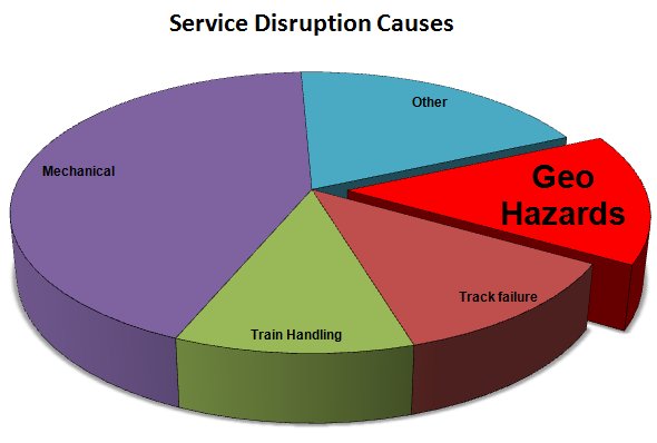
Historically, railway ground-hazard management was reactive: crews responded to washouts, slides, and rockfalls as they occurred. Beginning in the 1980s, the industry moved progressively toward a proactive posture, and by the mid-1990s several Class I railroads had formalized a Natural Hazard Risk Management system (CN's dates to 1995; its 1998 “Grade and Slope Stabilization Engineering and Management Protocol” combined previously separate hazard-management practices into one system). The driver was not only safety — though safety is the primary driver — but recognition that geo-hazard incidents, while less frequent than mechanical or track-related service disruptions, carry a disproportionately high average cost per event (see §17.9).
Soil and terrain conditions across a rail network trace directly to depositional history: understand how the ground was formed, and the likely failure mode follows. Glacial lake deposits and fine-grained ice deposits (silts and clays) dominate in prairie/plains terrain; coarser glacial till reflecting volcanic or sedimentary parent material dominates in shield and mountain terrain; and major river corridors bring their own flood and scour exposure wherever the alignment parallels or crosses them. A regional geotechnical specialist assigned to a defined territory — tracking conditions specific to that area's characteristic hazards (debris flows, retrogressive earthflows, rockfalls, rotational slumps) — is standard practice precisely because hazard character is so terrain- and geology-dependent.
Two concepts recur throughout this chapter and should be stated up front. Zero risk is impossible. Destabilizing forces are always active, conditions are dynamic, and many triggering events are unpredictable — an active warning system and a conservative shutdown decision the night before did not prevent the November 2012 rock shed collapse described in §17.4. These risks are also not simple “Acts of God” (force majeure — an influence not capable of being controlled, such as an earthquake). Risk can be significantly reduced over time through a proactive R.M. program, applied consistently rather than only after an event. No railroad is luckier than another; every network takes geo-hazard hits. What distinguishes a well-run program is a track record of mitigating impact, limiting losses, and recovering rapidly.
Profillidis observes that railways have tended to spend their improvement effort on the superstructure (rail, ties, ballast, subballast), while many of the problems that show up there are traceable to the subgrade. He also notes that early subgrade practice was borrowed from highway engineering: useful experience, but highway specifications applied literally did not fit the particular loading of a railway.
He distinguishes two situations. On a new line, subgrade design follows from axle load, tonnage, tie type and ballast thickness, together with soil type, hydrogeology and strength. On an existing line, the bottom of the subballast and the top of the subgrade have become a compact zone that should be disturbed as little as possible. Interventions should be limited to locations with demonstrated problems and timed with periodic maintenance, and the choice between improving the subgrade and thickening the ballast should rest on a technical and economic comparison.
The subgrade must let trains run safely at line speed, carry the axle loads, and minimize future maintenance cost. It does so by limiting settlement of the foundation and fill, staying mechanically stable under train loads, shedding rain and groundwater quickly, and not deteriorating over its working life.
Figures · click to zoom
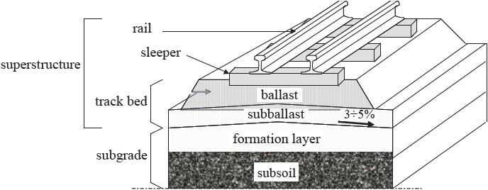
After Profillidis (2014), §7.2 and §9.1, Fig. 7.1. Full reference under Supplemental Sources.
This equation is the working tool for the decision every field engineer eventually faces: can a train safely run over a section of track affected, or potentially affected, by a geo-hazard event? A hazard that would rate as only moderate in isolation can still produce an unacceptable risk if the consequence of failure is severe — for example, a coastal slope where a blocked culvert forces ditch water through an embankment, causing a failure that leaves a near-vertical face and a long drop to open water below, with passenger service running over it. The hazard itself might not be rated severe; the consequence of a failure at that specific location is catastrophic, and the risk decision follows from the product, not either factor alone.
A related concept is the Factor of Safety (FoS): the forces holding a slope or embankment up should be at least 50% greater than the forces working to make it fail (FoS ≥ 1.5). At FoS near 1.0, failure becomes likely once any additional load — such as a heavy train — is added; even where the probability of failure is only moderate, a catastrophic consequence can still make the aggregate risk unacceptable.
The international disaster-risk community breaks the same equation into named components. UNDRR, through its PreventionWeb knowledge platform, describes disaster risk as the likelihood of loss of life, injury, destruction or damage over a given period. That risk arises when a hazard interacts with people and assets that are exposed and vulnerable to it, and it is written Risk = Hazard × Exposure × Vulnerability. The railway term “Consequence & Vulnerability” is the product of the last two: a failure has consequences only where something of value is in its path and cannot withstand it.
| Component | UNDRR meaning | On a railway corridor |
|---|---|---|
| Hazard | A process, phenomenon or human activity that can cause loss of life, injury, property damage, social and economic disruption or environmental degradation. Hazards may be natural, human-induced (anthropogenic) or socio-natural in origin. | The landslide, hydraulic-erosion and subsidence hazards of §1.3. Many are socio-natural: a cut steepened during construction, a blocked culvert, a beaver dam, or drainage altered beyond the right-of-way. |
| Exposure | The presence of people, infrastructure and other tangible assets in hazard-prone areas. | Track, roadbed, bridges and culverts within reach of the hazard; the trains, crews, passengers and commodities that pass the site; traffic density; and the length of corridor crossing active terrain. Railway exposure is linear and continuous (§1.1). |
| Vulnerability | Conditions set by physical, social, economic and environmental factors that make an asset or system more susceptible to a hazard’s impact. | Embankment condition and factor of safety, drainage and culvert capacity, ballast fouling, foundation type, line speed, train type (passenger, hazardous materials) and the lack of alternate routes. |
| Capacity | The strengths, attributes and resources available to an organization to manage and reduce risk and strengthen resilience (UNDRR terminology). | Track patrols and inspections, slide-detector fences and instrumentation, weather and GIS alerts, BAHA surveys, the Grade & Slope Stabilization Program, trained staff and emergency response. Capacity lowers vulnerability and shortens how long exposure lasts after an event. |
Three points follow for field practice. First, a hazard on its own is not a loss. The Gaspé-type embankment rates high because of what sits on and below it, not because the slope process is unusual. Second, each measure in the risk control hierarchy (§1.9) acts on a specific component. Stabilization reduces the hazard. Relocation and protection structures reduce exposure. Drainage repair and strengthening reduce vulnerability. Detection, warning and slow orders build capacity. Third, risk changes over time. Heavier axle loads, more traffic and new passenger service raise exposure. Aging culverts and fouled ballast raise vulnerability. Changing rainfall extremes alter the hazard itself. A site’s rating therefore has to be revisited on a schedule, not filed.
After UNDRR, PreventionWeb, “Understanding disaster risk: Components of risk,” and UNDRR terminology on disaster risk reduction. Full reference under Primary sources.
CAN/CSA-Q850-97, Risk Management: Guidelines for Decision-Makers, frames risk management as an iterative, cyclical process rather than a one-time assessment. Applied to railway ground hazards, the process comprises six stages, with a seventh — Risk Communication — running throughout and feeding information back into the first:
| Stage | Purpose |
|---|---|
| Initiation | Kick off the process for a given hazard, site, or network segment; identify the R.M. team and a responsibility matrix |
| Preliminary Analysis | Identify, categorize, and characterize ground hazards; develop risk scenarios for each category |
| Risk Estimation | Analyze frequency and consequence for each scenario; screen for the greatest loss exposure |
| Risk Evaluation | Weigh the assessed risk against acceptable thresholds using a risk resolution matrix; set mitigation priorities |
| Risk Control | Select and apply proactive mitigation measures, in order of preference: reduce the hazard, protect the track, or warn trains |
| Action / Monitoring | Implement controls; monitor conditions and control effectiveness; feed results back into Preliminary Analysis |
Risk involves three key issues under this framework, and the third is easy to under-weight: the frequency of the loss, the consequence of the loss, and the perception of the loss by the affected stakeholder. Understanding stakeholder perception is treated as being as important as frequency or consequence, because it drives whether operating personnel, regulators, and the public accept a given risk-control decision. “Stakeholder” here means any individual, group, or organization able to affect, or that believes it may be affected by, a decision — for a railroad, primary stakeholders include the operating personnel whose duties bring them into proximity with ground hazards day to day.
Reference graphics · click to zoom
In the field the risk equation is a decision tool. It answers whether a train can safely run over track that a geo-hazard has affected, or may affect. The course’s Gaspé example makes the point: a blocked culvert forced ditch water through an embankment above a roughly 100-ft drop to the ocean, on a passenger route. The hazard alone might not have rated severe, but the consequence made the decision obvious. The related factor-of-safety rule of thumb is that the forces holding an embankment up should exceed the driving forces by at least 50% (FoS ≥ 1.5). Where the consequence is catastrophic, even a moderate probability of failure is unacceptable.
Figures · click to zoom
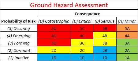
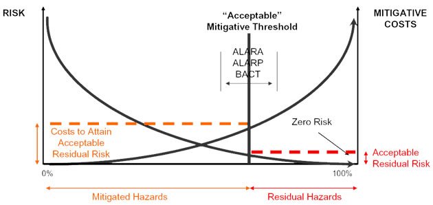
After Geotechnology for Railroaders Program, Module 1; §04. Full reference under Supplemental Sources.
Step one of the R.M. process is identifying exactly what the potential hazards are: inventory every geo-natural event that can affect the track, then sort them into manageable main categories before considering the triggering perils (rainfall, snowmelt, freeze/thaw, seismic events) separately. Railway ground hazards divide first between landslides and hydraulic erosion, with subsidence hazards — limited to track-foundation failures specifically — forming a third category.
| Category | Representative Hazards | Typical Risk Rating |
|---|---|---|
| Landslide Hazards | Rock slide, debris flow, sensitive-clay slide/spread, downhill and uphill instability | High |
| Hydraulic Hazards | Surface (runoff) erosion, river flow & wave erosion, internal seepage erosion; washouts including beaver-related failures | Elevated |
| Subsidence Hazards | Ballast failure (mud spots), foundation failure, muskeg punching, frost heave, culvert failure, buried-timber decay, burrowing animals | Guarded |
Subsidence hazards make up roughly 80% of what track patrollers actually encounter day to day, even though landslide events tend to be the larger and more visually dramatic failures — a distinction worth internalizing, because it means routine patrol vigilance and dramatic-event response are two different disciplines that both need to be funded.
Within landslide hazards, following Cruden & Varnes (1996), the next distinction is by material type — rock, debris, earth, or granular versus cohesive/organic soil (including engineered fill) — crossed with movement type: fall, topple, slide, spread, or flow. Snow and ice classifications extend the same scheme to avalanche hazards. The non-cohesive/cohesive split matters because the two soil families fail by different mechanisms and under different triggers: non-cohesive materials are liquefaction-prone when saturated, while the notable exception on the cohesive side is the behavior of highly sensitive and quick clays, which can fail with very little precursor movement.
Within hydraulic erosion, the corresponding first split is between seepage erosion and surface-flow erosion, again because the failure characteristics and contributing factors differ significantly between the two mechanisms. The full inventory tracked under this category includes: surface flow (runoff) erosion, stream and wave erosion, underground (seepage) flow erosion, slope wash, gully erosion, piping, erosion around culverts, channel aggradation and degradation, local and contraction scour, ice/log-debris jams, bank erosion, encroachment, avulsion, flooding, and beaver dam failure.
Within subsidence, the governing distinction is behavioral rather than material: progressive settlement (consolidation, compression and active clays, subgrade dynamic liquefaction, subgrade bearing-capacity failure, ballast mud spots) versus sudden collapse (piping voids, culvert failure, failed buried pipelines/utilities, liquefaction, voids in buried rock fill, burrowing animals, tunnelling and mining subsidence, decay of buried timber, collapsing soils over subsurface cavities). Uneven track and a “muddy” surface condition can look identical regardless of which of these three or four root causes is actually responsible — diagnosing the true cause, not just treating the symptom, is essential before selecting a repair.
| Region | Terrain | Predominant threats |
|---|---|---|
| West | Mountains | Rock fall, debris flow, earth slides |
| South | Level terrain | Storms, hurricanes, floods, scour, earthquakes |
| East | Hills and level terrain | Washouts, earth slides, soft soils, coastal erosion |
| Central | Level terrain, glacial and lake-bed deposits | Floods, earth slides, silt–sand lake and river-delta deposits |
Terrain behavior traces back to how the ground was deposited. Glacial-lake clays and silty tills dominate the Prairies; coarser tills derived from volcanic and sedimentary rock dominate the Shield and the mountains. In the U.S., the Missouri, Ohio and Mississippi crossings bring their own flood and scour exposure. Subsidence hazards make up about 80% of what track patrollers actually encounter, even though landslides are the more spectacular events.
Figures · click to zoom
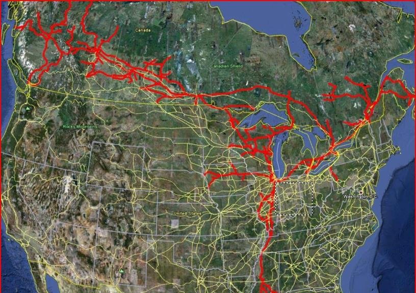
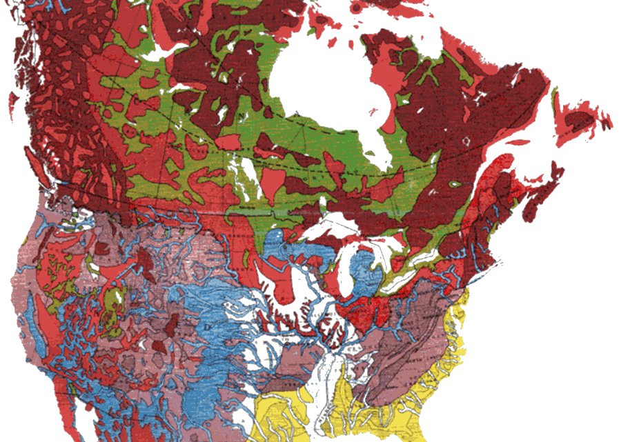
After Geotechnology for Railroaders Program, Module 1; §03, §05. Full reference under Supplemental Sources.
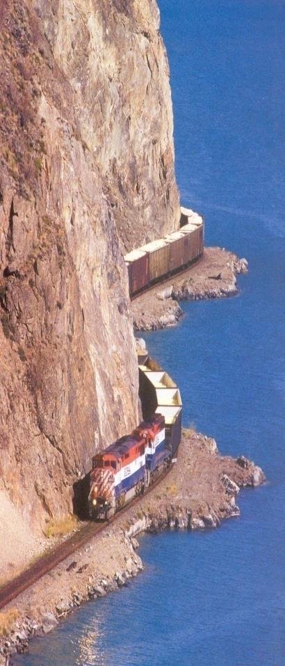
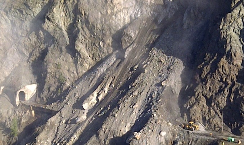
Typical risk rating: High. Rail lines in steep, geologically active terrain (mountainous western corridors are the classic case, though the same hazard families occur wherever the alignment cuts through active slopes) often run close to steep rock faces of poorer-quality rock, sometimes protected by rock sheds and post-and-wire rockfall warning systems that trigger an alarm so trains can slow and inspect for an obstruction. A dedicated rockfall hazard-and-risk assessment program (see §17.7) tracks and prioritizes rockslide-prone slopes at the scale of thousands of individual sites, continuously monitored.
Risk rating: Severe. Crews working near an active post-and-wire rockfall warning system observed rockfall activity above normal levels and shut the line down for the night as a precaution. The next morning, the rock shed was found crushed, with rock debris covering the entire track. Clearing crews began digging despite concern about a large overhanging rock they believed would hold — until it moved. Spotters can buy workers time to react, but predicting exactly when and how a slope will move remains extremely difficult; the loose rock was ultimately blasted to stabilize it before clearing could safely continue. Clearing the line took six days, with additional material continuing to fall throughout the excavation.
Takeaway: an active warning system and a conservative shutdown decision made the night before still did not prevent the shed's collapse. Zero risk is impossible; the goal of a risk-management program is proactive reduction of consequence and exposure, not elimination of hazard.
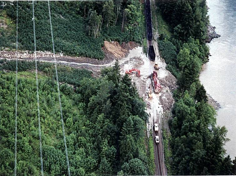
Debris flows (High). Debris flows accumulate high above the track over years as material builds up in a source area that is often not visible from track level; a storm event then releases the accumulated material downslope, and it can reach the track as far as one to two miles from where it originated. Because the source area is frequently hidden from the patroller's normal sightline, confirming what is actually happening upslope sometimes requires climbing to the source or an aerial overflight before a track-level event occurs.
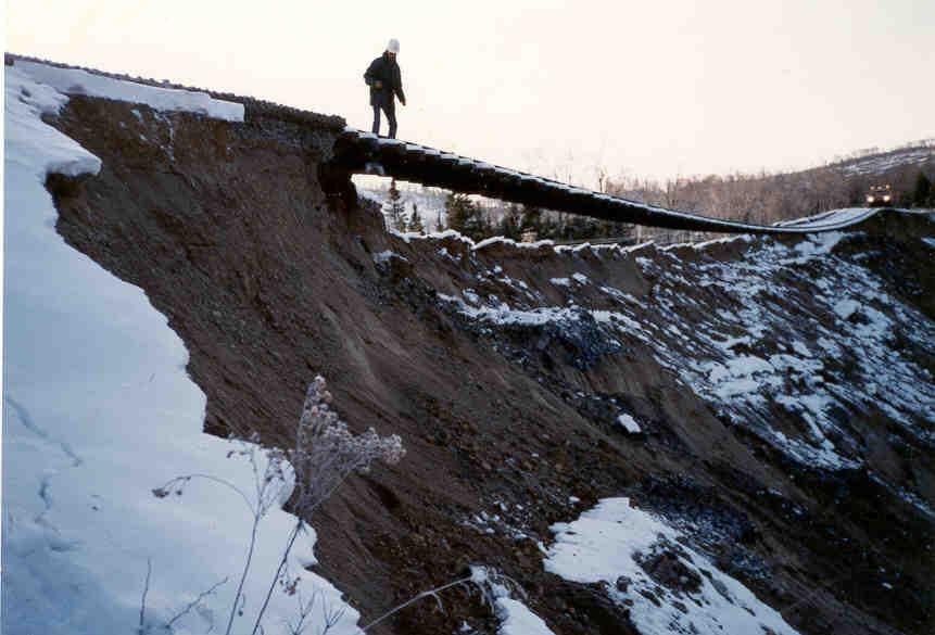
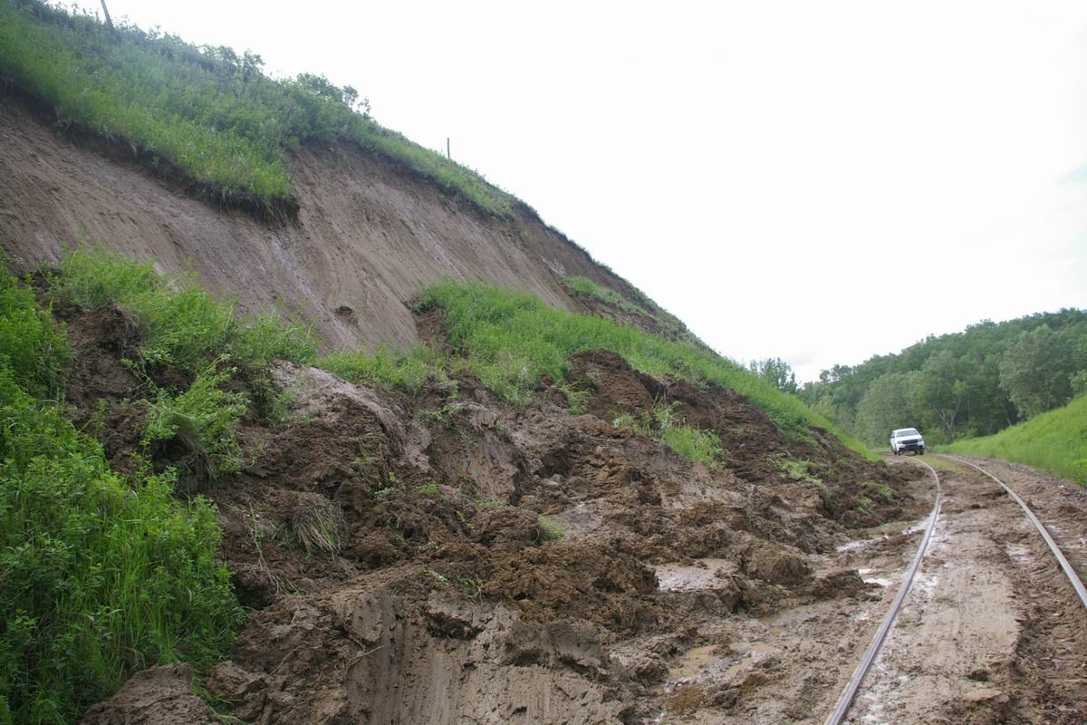
Earth slides and embankment failures (High). Sensitive clay terrain produces a distinctive and dangerous hazard: retrogressive earthflows that begin beside a river or waterway and cascade into successive earthflows as the clay liquefies, often with very little precursor movement — capable of rapid, catastrophic failure over tens of feet of clay and taking track out of service for months at a time. Fissures on the flank and a head scarp are the early warning signs to watch for. Landslides are not limited to slopes below the track, either: a non-cohesive surficial failure can send mud pouring over the track from a slide originating above it, a reminder that uphill terrain deserves the same scrutiny as downhill terrain during patrol.
A landslide awareness handbook written for non-specialists lists warning signs that transfer directly to track patrol and roadmaster training:
Delayed failures are real. Geological Hazards notes that some English railroad cuts failed 60–70 years after excavation as slow creep progressed to failure. It recommends residual rather than peak strength for investigating or analyzing such slopes (see Chapter 13 for fully softened versus residual strength).
Volcanic and glacial outburst hazards. At Tangiwai, New Zealand (December 1953), the collapse of a crater-lake rim on Ruapehu sent a flood down the Whangaehu River that picked up debris and became a mudflow up to about 20 ft high. It struck a railroad bridge and partly carried it away, leading to the derailment of the Wellington–Auckland express and the loss of 154 lives. Upstream impoundments — crater lakes, glacial lakes, landslide dams and beaver ponds — belong in the corridor hazard inventory even when they are far from the track.
Source: Meyer, P. Landslide Hazard Manual — Trainer’s Handbook. Engineering for the World · Bolt, B. A., Horn, W. L., Macdonald, G. A. and Scott, R. F. (1977). Geological Hazards, 2nd ed. Springer-Verlag
Rock shed collapse, November 2012 (rated Severe). Crews working near a rock shed shut the line down for the night when a post-and-wire warning system showed more rockfall than usual. By the next morning the shed had been crushed and rock covered the track. Clearing took six days, more material fell as excavation proceeded, and an overhanging block that crews expected to hold eventually had to be blasted.
Debris flows start from material that builds up high in a drainage for years and is released by a storm. They can reach the track 1–2 miles from their source, which is often invisible from the track. Sensitive-clay earthflows in Eastern Canada retrogress from a riverbank with little warning; at St-Fabien about 80 ft of clay liquefied and the track was out of service for six months. Watch for fissures on the flanks and head scarp. At Qu’Appelle, Saskatchewan, a slide from above the track poured mud across it, so check uphill terrain as well as downhill.
Figures · click to zoom
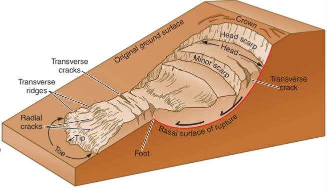
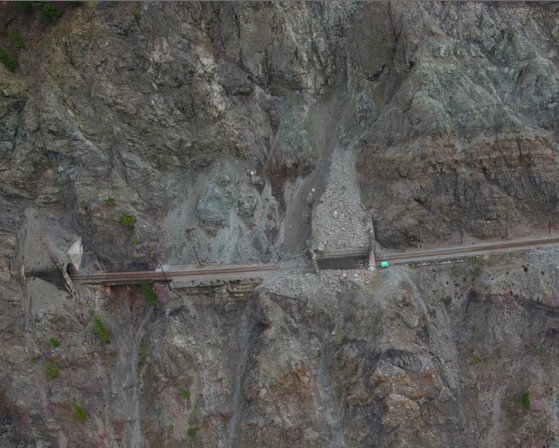
After Geotechnology for Railroaders Program, Module 1; §06. Full reference under Supplemental Sources.
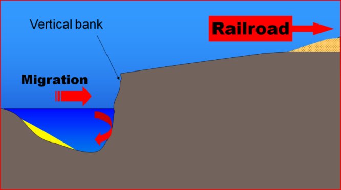
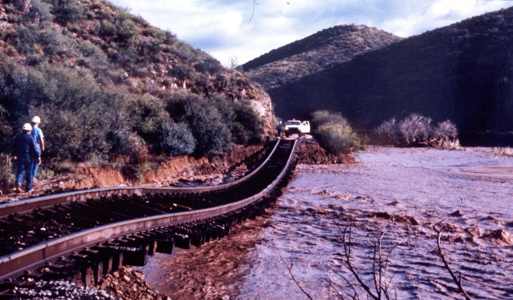
Typical risk rating: Elevated. Hydraulic hazards split first into surface erosion and underground (seepage) erosion, and secondarily by mechanism: stream and wave erosion, slope wash, gully erosion, piping, culvert erosion, channel aggradation/degradation, local and contraction scour, ice/log-debris jams, bank erosion, encroachment, avulsion, flooding, and beaver-dam failure. Two purpose-built risk-assessment tools track the highest-consequence versions of this category: a River Attack Risk Assessment for lateral stream migration and bank/pier attack, and a Beaver Activity Hazard Assessment for the beaver-related subset (see §17.7).
Scour — the action of flowing water eroding soil — deserves particular attention while patrolling: watch for it around river bends (where streambeds scour at the outer radius and deposit on the inside radius) and under piers, since scour can also trigger a landslide as a secondary event once the toe support at the base of a slope is removed.
Reference graphics · click to zoom
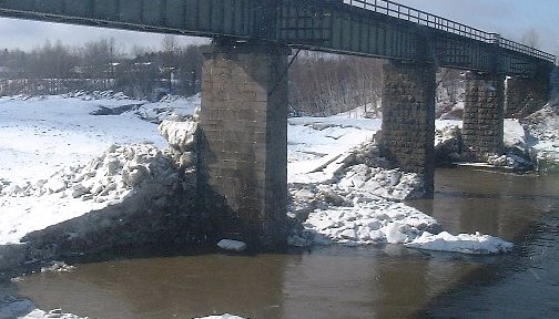
Risk rating: High. Ice buildup at a river bridge displaced an entire pier by one to two feet. The initial proposal — a large rock berm to stop the advancing ice — would have effectively dammed the river and caused significant environmental damage. The better solution, drilling through the piers and re-anchoring them into the underlying rock, avoided that impact entirely.
Takeaway: don't improvise a fix until the root cause is understood. A structurally obvious symptom (a displaced pier) can have a root cause (advancing river ice) whose most available fix (a berm) creates a worse secondary problem than the one it solves.
Beaver ponds attenuate floods while they hold, but a failed dam releases the stored water at once. Welsh (2012, after Butler and Malanson, 2005) compiles documented failures. The railway cases show why the beaver assessment described in §1.8 exists:
Table 1-S1. Documented beaver-dam failures affecting railways and people (condensed)
| Event | Consequence |
|---|---|
| Williston, Vermont (reported 1984) | Outwashed beaver dams damaged a drainage culvert and railroad embankment; Amtrak passenger train derailed — 5 killed, 149 injured |
| Nokina, Ontario (TSB Canada, 1994) | Track-bed failure from sudden drawdown after a beaver dam failed; CN freight derailed — 2 crew killed, 1 seriously injured |
| Central Michigan (reported 2003) | Beaver dam collapse washed out a culvert under the railway; freight derailed, 2 employees injured |
| Oglethorpe County, Georgia (Butler, 1989) | Outburst flood killed 4 people and floated a truck |
| Central Alberta, June 1994 (Hillman, 1998) | Flood wave 3.5 times the maximum discharge recorded in 23 years; five downstream gauging stations destroyed |
Two mechanisms recur: overtopping and washout of a culvert or fill by the outburst, and rapid drawdown of a pond impounded against the embankment, which leaves the fill saturated with its external support removed (Chapter 13, §13.8).
Source: Welsh, S. B. (2012). Geomorphic Changes Following Beaver Dam Failure and Abandonment. Plan B report, Utah State University (Table 5, modified from Butler and Malanson, 2005)
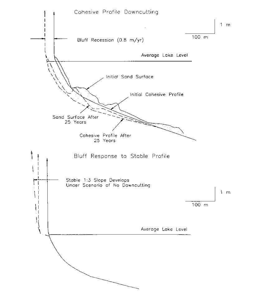
Lines along the Great Lakes, New England and the Pacific run on or behind eroding bluffs. USACE EM 1110-2-1810 reports average U.S. shoreline erosion of about 1.3 ft/yr (Atlantic 2.6 ft/yr; Gulf 6 ft/yr, up to 14 ft/yr in Louisiana; Pacific essentially stable where the shore is hard rock). Cliff retreat is significant in the Great Lakes, Pacific, New England and New York. On cohesive (clay or till) shores, erosion is irreversible: waves abrade and cut down the nearshore clay, which lets larger waves reach the toe, and the bluff steepens and slumps (Figure 1-S2). A thin sand cover can accelerate abrasion, but once the sand becomes thick enough it protects the clay and recession stops. Where waves remove toe debris faster than it accumulates, the bluff retreats quickly with a steep face. Higher lake levels are expected to accelerate Great Lakes recession, while California cliff retreat is episodic and driven by severe winter storms, runoff and groundwater. For risk scoring, estimate the time until the recession line reaches the track, not just the current setback; for protection options, see revetment design in Chapter 16.
Source: U.S. Army Corps of Engineers (1995). Coastal Geology. EM 1110-2-1810
The hydraulic inventory tracked includes surface runoff, stream and wave erosion, underground flow, slope wash, gullying, seepage, piping, erosion around culverts, aggradation and degradation, local and contraction scour, ice and log jams, bank erosion, encroachment, avulsion, flooding and beaver dams. Scour can also trigger a landslide as a secondary event.
Pier displacement near Quebec City (rated High). Ice buildup moved an entire pier 1–2 ft. The first proposal, a large rock berm against the ice, would have dammed the river. Instead the piers were drilled and re-anchored into rock. The lesson: do not improvise a fix before the root cause is understood.
Figures · click to zoom
After Geotechnology for Railroaders Program, Module 1; §07. Full reference under Supplemental Sources.
Case study: 1.15.1 St Lucia riverbank slide: back-analysis gives probabilities, and the repair length (Look 2023), in §1.15 Case Studies.
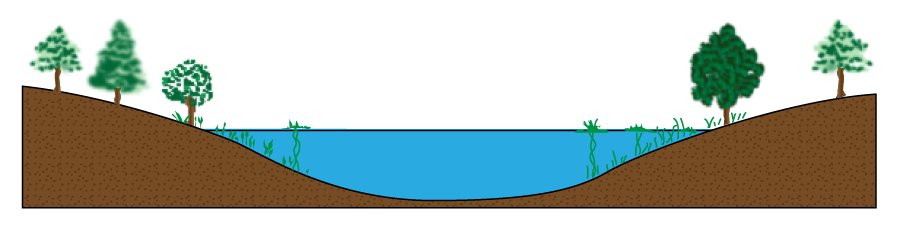
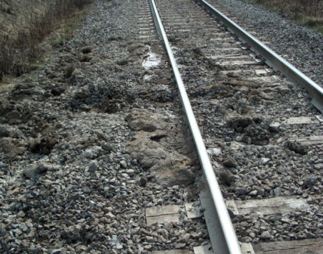
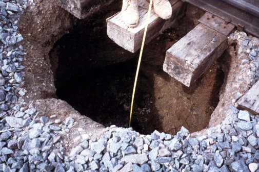
Typical risk rating: Guarded — but the category responsible for roughly 80% of what patrollers actually encounter, precisely because it is the least dramatic and most chronic of the three families. Subsidence hazards split into progressive settlement (consolidation, active-clay compression, subgrade dynamic liquefaction, subgrade bearing-capacity failure, ballast “mud spot” failure) and sudden collapse (piping voids, culvert failure, failed buried utilities, liquefaction, voids beneath large rock fill, burrowing-animal tunnels, mining/tunnelling subsidence, decayed buried timber, collapse over subsurface cavities).
Risk rating: Elevated. A peat bog is, in effect, an old lake bed sitting on vegetation, acting like a sponge. As buried wood decays, sink holes form and the track above begins to sink. Under train loading, stress radiates straight down through the peat, building up water pressure that forces material upward and creating a void beneath the track that then collapses.
Documented fixes and their track record:
Takeaway: a “muddy track” surface symptom can have three or four distinct root causes; the fix has to match the diagnosis, not the symptom, and no single repair method solves every muskeg site.
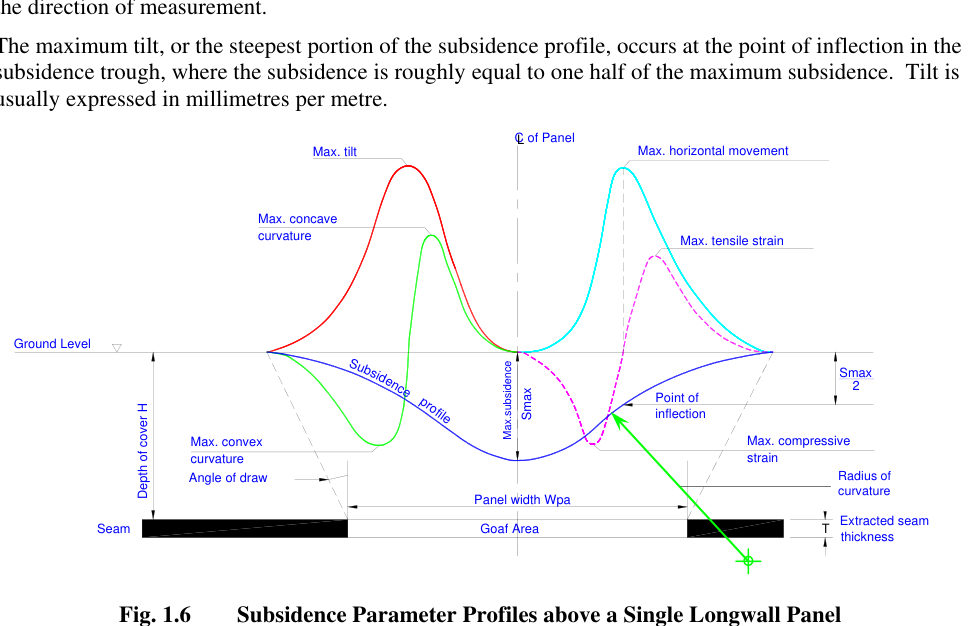
Longwall mining removes a whole panel of coal — typically about 500–1,000 ft wide, 3,300–11,500 ft long and 6.6–16 ft thick, advancing about 164–330 ft per week. The roof caves behind the face, and a subsidence trough forms at the surface soon after mining. The U.S. EIA reports planned longwall subsidence of about 4–6 ft, or 60–70% of the extracted height. Movement diminishes quickly after a few months but continues for years. The trough extends beyond the panel by the angle of draw, typically 10–35° from vertical (Figure 1-S1).
For track, the damaging parameters are the derivatives of the trough rather than the settlement itself. Tilt (the first derivative) is greatest at the inflection point, where settlement is about half the maximum. Curvature (hogging over the panel edges, sagging toward the center) and horizontal strain follow: tension over the edges, compression toward the middle. Horizontal displacement can exceed vertical displacement where subsidence is small. As the face passes beneath the line, a given point is pulled toward the void and goes through tension and then compression, so rail stress, joint gaps, track geometry and culvert or bridge alignment need monitoring as the face passes, not just a before-and-after survey.
Room-and-pillar mining is less predictable. Pillars can fail during mining or decades after abandonment, producing pits (typically 6–8 ft deep and 2–40 ft across, most under 16 ft, with steep or bell-shaped walls) or broad sags as large as a mine panel. A roof failure 160 ft down caused minor surface subsidence more than 75 ft beyond the undermined area. Old mine maps, the angle of draw and mine-subsidence insurance or regulatory records belong in the desk study for any corridor in coal country.
Old railway tunnels are a related subsurface hazard. Papers in Geotechnical Risk in Rock Tunnels attribute deterioration in old tunnels to decompression of the rock around the cavity from historical construction methods, voids behind the lining, open masonry joints, water, and rock-mass loading on the lining. They also note that most reported underground collapses involved railway or subway tunnels.
Source: Mine Subsidence Engineering Consultants (2007). Introduction to Longwall Mining and Subsidence, Rev. A · U.S. Energy Information Administration (1995). Longwall Mining. DOE/EIA-TR-0588 · Campos e Matos, A., Ribeiro e Sousa, L., Kleberger, J. and Lopes Pinto, P. (eds.) (2006). Geotechnical Risk in Rock Tunnels. Taylor & Francis/Balkema
| Progressive settlement | Sudden collapse |
|---|---|
| Consolidation; compression and active clays; subgrade dynamic liquefaction; subgrade bearing-capacity problems; ballast failure (mud spots) | Piping voids; culvert failure; buried pipelines and utilities; liquefaction; voids in buried rock fill; burrowing animals; tunnelling and mining; decay of buried timber; collapsing soils over cavities |
“Muddy track” may have three or four different root causes, so diagnose before repairing. Documented muskeg fixes have mixed records. A trench of filter cloth, gravel and woven geotextile under sub ballast and ballast, which redirects water out the sides, worked about 60% of the time. French drains lowered the local water table 2–3 ft. Cement powder filled sink holes, but water sometimes bypassed the treated hole.
Figures · click to zoom
After Geotechnology for Railroaders Program, Module 1; §08. Full reference under Supplemental Sources.
A risk scenario is a sequence of events with an associated frequency and consequence, typically combining one or more ground hazards (conditions) with one or more perils — the triggering events that convert a latent condition into a loss. Perils tracked in practice include intense rainfall, floods, high stream flows, rapid snowmelt, rain-on-snowpack, elevated groundwater seepage, prolonged rainfall, freeze/thaw cycling, and seismic activity. Symbolically: Ground Hazard(s) × Peril(s) → Loss.
A representative scenario: erosion at the toe of a slope removes support (a hazard); this over-steepens the overall slope, raising the potential for an earth slide (a new hazard resulting from the first); an intense rainstorm then hits the location (a peril), raising pore-water pressure in the slope and triggering the earth slide; the grade beneath the track slips away, and a train traversing the site derails — the consequent loss.
Loss exposures fall into five categories: personnel (illness, injury, or fatality), property (equipment, commodities, track, roadbed, facilities), liability (arising from torts, statutes, or criminal law), environmental, and income (service disruption and lost market share). At the Risk Estimation stage, frequency may be based on historical incident data (with the inherent assumption that future conditions mirror the past), published peril-frequency data (climatic or seismic), or, where no relevant historical data exists, methods such as fault-tree or event-tree analysis. Consequence is normally measured in injuries, property-damage value, cleanup cost, business loss, and environmental impact; where insufficient data exists, expert judgment must substitute for statistics.
A subtlety worth flagging explicitly: a given site may show low individual risk, yet the aggregate risk across a rail corridor can be high if a series of hazard locations, each individually low-risk, are coupled with a high probability of a shared triggering peril — this is particularly true for climatic and seismic perils that can affect many sites simultaneously, and it requires a more sophisticated, corridor-level view than any single-site assessment provides.
Once frequency and consequence are estimated, a risk resolution matrix — probability of occurrence crossed with consequence severity — sorts scenarios into Unacceptable, Tolerable with Mitigation, and Tolerable categories, providing a consistent basis for prioritizing which sites receive attention first and for communicating that prioritization to stakeholders:
| Probability \ Severity | Catastrophic | Critical | Marginal | Negligible |
|---|---|---|---|---|
| Frequent | Unacceptable | Unacceptable | Unacceptable | Tolerable w/ mitigation |
| Probable | Unacceptable | Unacceptable | Tolerable w/ mitigation | Tolerable w/ mitigation |
| Occasional | Unacceptable | Tolerable w/ mitigation | Tolerable w/ mitigation | Tolerable |
| Remote | Tolerable w/ mitigation | Tolerable w/ mitigation | Tolerable w/ mitigation | Tolerable |
| Improbable | Tolerable w/ mitigation | Tolerable w/ mitigation | Tolerable w/ mitigation | Tolerable |
Adapted from the American Public Transit Association's Manual for the Development of System Safety Program Plans for Commuter Railroads, as applied within the CAN/CSA-Q850-97 risk-management framework.
Case study: 1.15.2 Brisbane 2010/11: landslides whose cost bore no relation to the damage (Look 2023), in §1.15 Case Studies.
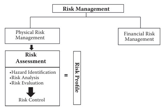
McKinnon (2012) divides physical risk management into risk assessment and risk control. Assessment has three steps: hazard identification, risk analysis and risk evaluation, which together produce a risk profile. Hazard identification is either comparative (checklists from codes, industry standards, or similar operations) or fundamental (structured study of how deviations could trigger hazards). Fundamental methods include HAZOP, a guide-word review by a multidisciplinary team; FMEA, which lists each failure mode of each component and its effect; FMECA, which adds a criticality ranking; fault tree analysis, which works downward from an undesired top event through logic gates to root causes; event tree analysis, which works forward from an initiating event through branching outcomes; and SWIFT (“so what if it happens?”) brainstorming. Past accident and near-miss records, critical task analysis and safety audits are further sources.
Risk analysis asks what could happen, how often and with what exposure, and how bad the outcome would be. A simple index multiplies probability × frequency × severity, each ranked 1 (low) to 4 (high). McKinnon distinguishes the maximum possible loss (all controls fail) from the maximum probable loss (controls work reasonably well) and recommends assessing the normal expectancy. Risk evaluation then weighs the cost of reduction against its benefit; risks are reduced until they are “as low as reasonably practicable” (ALARP). Control options are the four Ts: treat (loss control), tolerate (finance the loss), transfer (insurance, usually for low-frequency, high-severity risks) and terminate (stop the activity).
For railroad work: The same structure fits ground-hazard scenarios. A fault tree from a top event such as “train encounters washed-out embankment” can trace the combinations of culvert blockage, rainfall above threshold and missed inspection; an event tree from “slope movement detected” can branch through alarm, slow order, track inspection and train stop. For field programs, use the comparative method (job briefing checklists) for routine drilling and the fundamental methods for unusual work such as excavation beside an active main track. Keep the distinction between possible and probable loss explicit when ranking sites, so worst-case scenarios do not swamp the ranking of everyday hazards.
Source: McKinnon, R. C. (2012). Safety Management: Near Miss Identification, Recognition, and Investigation. Boca Raton, FL: CRC Press (Taylor & Francis), pp. 75–87. Summarized and paraphrased; figures reproduced for internal reference. Full reference under Supplemental Sources.
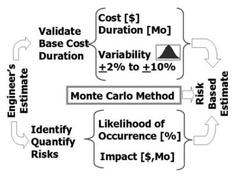
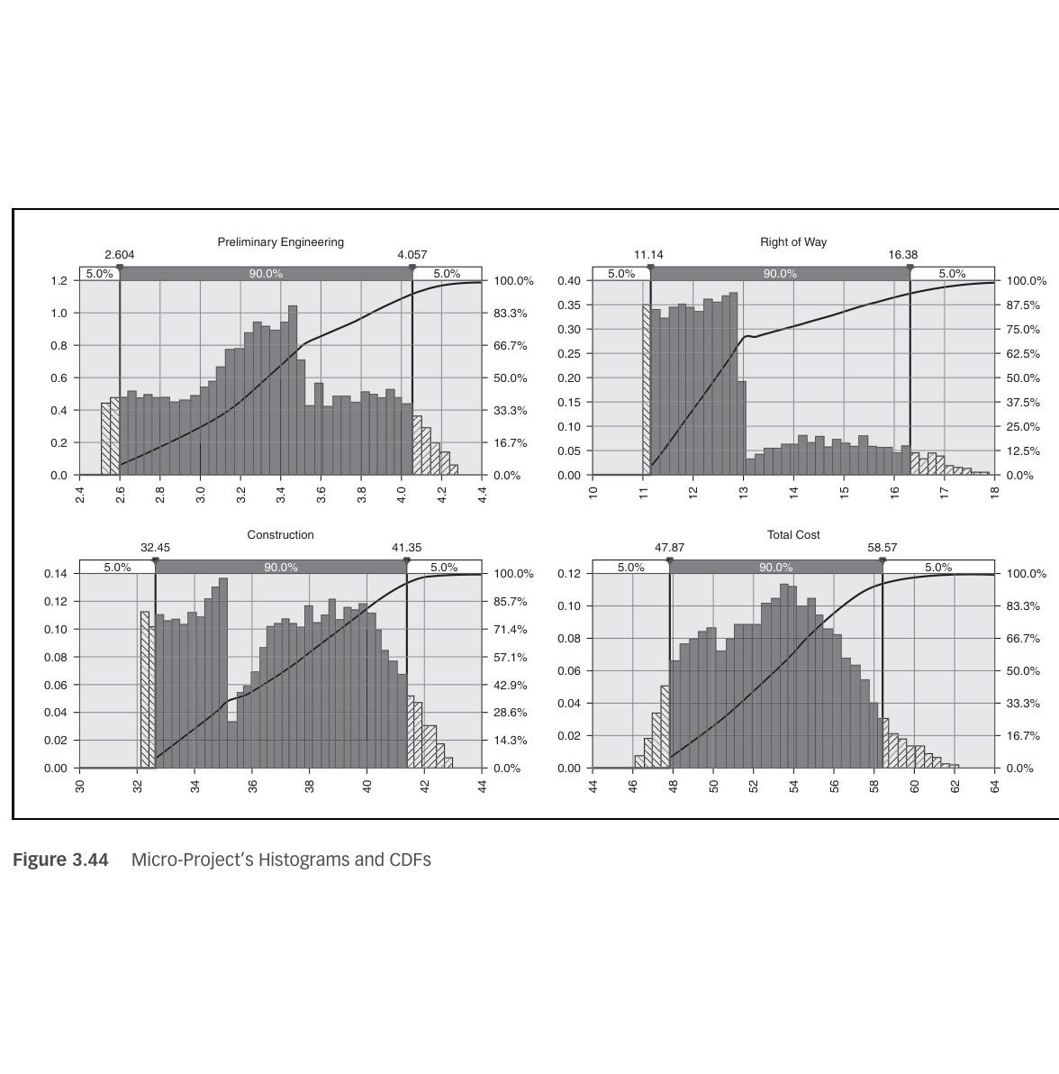
The hazard-risk estimation in this chapter rates the likelihood and consequence of ground events affecting the operating railway. Cretu et al. apply the same logic to a project’s cost and schedule in what they call the risk-based estimate (RBE). First, the engineer’s estimate is validated by a reviewer with no stake in the project. Contingencies hidden in unit prices are removed, and a design allowance is kept for undefined items. What remains is the base, meaning the cost and duration if the project goes as planned. The base receives a symmetrical variability, typically ±2 to ±10 percent, modeled with a symmetrical Pert distribution. Anything that would skew the outcome is captured instead as a discrete risk event with a probability of occurrence and a three-point impact (low, most likely, high). Threats and opportunities are both listed. Monte Carlo simulation then samples the base and each risk thousands of times to produce percentile tables, histograms, cumulative curves and tornado charts.
The authors use a three-activity “micro-project” to show the mechanics. The base costs are $2.5–3.5 million for engineering, $11–13 million for right of way and $32–35 million for construction. The risk events are a 50 percent chance of +$0.5–0.8 million on engineering, a 30 percent chance of +$1–5 million on right of way and a 66 percent chance of +$2–8 million on construction. Against a $54 million budget, the simulation gives about a 60 percent chance of staying within budget. The sum of the component 90th percentiles exceeds the 90th percentile of the simulated total by about 5 percent, because percentiles do not add; only means do. They recommend probability steps of 5, 25, 50, 75 and 95 percent, with 50 percent reserved for “no idea.” They also advise keeping the analysis to the 15–20 risks that can actually move the result.
For railroad work: Use the RBE when a slide repair, embankment rebuild or culvert replacement needs a defensible budget and track-outage duration. Keep the base to quantities that are known. Model as discrete events the things that make railroad projects run long: a deeper failure surface than assumed, unsuitable foundation soil requiring extra undercut, a lost or shortened track window, a weather-driven reactivation during construction, and utility or signal cable conflicts. Then report the funding level at a stated confidence, for example P70, instead of a single number.
Source: Cretu, O., Stewart, R. and Berends, T. (2011). Risk Management for Design and Construction. Hoboken, NJ: John Wiley & Sons, pp. 42–45, 63–66, 84–90. Summarized and paraphrased; figures reproduced for internal reference. Full reference under Supplemental Sources.
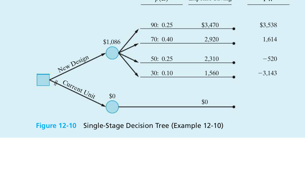
Sullivan et al. present decision trees for problems with uncertain outcomes or decisions made in sequence. The conventions are:
At a chance node the value is the expected present worth, E(PW) = Σ p × PW. In Example 12-10 (Figure 12-10), a design costs $8,600 more and has four possible levels of performance. Their PWs are $3,538, $1,614, −$520 and −$3,143, with probabilities 0.25, 0.40, 0.25 and 0.10. E(PW) is $1,086, which is above zero, so the design is adopted even though two of the four outcomes lose money. A second, deterministic example shows that discounting can reverse a replacement decision. At 25% interest, keeping the old asset becomes the better choice at every decision point.
The book’s Problem 12-6 asks how high to raise a levee. Each design level has a capital cost and an annual probability that a storm surge overtops it, and an overtopping causes about $100 million of damage. Working the problem, with costs financed on 30-year bonds at 6% (capital recovery factor 0.0727), total expected annual cost is capital recovery plus probability × damage:
The Category 4 design has the lowest total. It is still the lowest if the damage is doubled to $200 million.
For railroad work: this is the risk equation of Section 1.2 put into dollars. For a culvert, scour, rockfall or slide site:
Where an investigation or a monitoring period could change the probabilities, build that as an earlier decision node. The tree then shows the value of the information before the money is spent.
Source: Sullivan, W. G., Wicks, E. M. and Koelling, C. P. (2015). Engineering Economy, 16th ed. Upper Saddle River, NJ: Pearson, pp. 530–535, 539–540. Summarized and paraphrased; figures reproduced for internal reference. Full reference under Supplemental Sources.
Because a Class I network can carry on the order of a thousand or more individually tracked rockslope and beaver-dam sites, a workable R.M. program depends on standardized tools that convert field observations into comparable, prioritizable scores rather than ad hoc judgment calls. Four tools recur across the industry:
| Tool | Purpose |
|---|---|
| Rockfall Hazard & Risk Assessment | Event-tree analysis assigning each catalogued rockslope a subjective probability of derailing a train; generates a derailment-hazard score used to prioritize and set inspection frequency across on the order of 1,000–1,500 tracked rockslopes |
| Beaver Activity Hazard Assessment (BAHA) | Scores the potential for beaver activity to disrupt track serviceability from ponded-water volume, dam condition, topography, and the ability of infrastructure to handle a sudden release; guides dam removal, nuisance-beaver control, and anti-reconstruction devices |
| Earthquake Notification System | Real-time link to a regional seismograph network; delivers immediate location/magnitude information to train control and specifies response actions (reduced speed or halt, pending field inspection) keyed to event magnitude |
| Weather Reporting & GIS | Contracted forecasting with near-real-time and antecedent rainfall reporting; increasingly paired with radar precipitation data and soil-moisture modeling on a fine spatial grid to flag elevated runoff and saturation potential before a peril event arrives |
An effective information-management system underpins all four: a relational database and GIS application maintaining a ground-hazard inventory across potentially thousands of sites, with each entry carrying site conditions, hazard type, potential trigger conditions, a subjective failure-rate and consequence assessment, the latest hazard/risk score, current priority, and proposed mitigation. This inventory is what makes the Preliminary Analysis and Risk Evaluation stages of the R.M. cycle (§17.2) repeatable rather than reinvented at every site.
The BAHA inspection notes (Ruel, 2008) describe how CN’s western territory was flown by helicopter with a GPS-linked laptop GIS, with a separate screen for back-seat observers:
Source: Ruel, M. (2008). MapInfo – BAHA Geo-hazard Inspection Instructions (helicopter inspection set-up and procedures)
Case study: 1.15.3 Regional landslide hazard zoning by GIS (Look 2023), in §1.15 Case Studies.
Risk Control is any conscious action — or documented decision not to act — that reduces the frequency, severity, or unpredictability of a loss. The preferred approach is always proactive mitigation of the loss exposure itself, which is almost always more cost-effective than absorbing the cost of a derailment or unplanned service disruption. In order of preference:
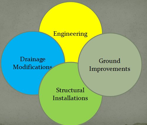
Once a site is prioritized through the risk-resolution matrix (§17.7), the applicable risk-control measure typically falls into one of four categories: Drainage Modifications, Engineering (regrading, retaining structures, rock reinforcement), Ground Improvements (see Chapter 17, Section 17.16 — Ground Improvement Technology Library), and Structural Installations (sheds, fences, nets, culvert replacement). The single most under-respected principle across every category is drainage: a railroad should invest roughly 3% of its operating budget on drainage and ditch maintenance, but in practice that spending competes with — and often loses to — rail and crossing work, until poor drainage becomes the problem that stops service.
Profillidis places maintenance and renewal decisions inside two cost concepts — the life-cycle cost of each component (from conception through operation to the end of its economic life) and life-cycle costing, the systematic economic evaluation of those costs over an analysis period — and inside a global performance concept known as RAMS:
For outsourced maintenance he recommends sensitivity analysis of the critical contract terms, confirming that both life-cycle cost and track quality improve, quantifying the probability of non-delivery, and identifying fallback solutions. These are the same questions a ground-hazard risk control should answer before it is selected.
After Profillidis (2014), §16.11. Full reference under Supplemental Sources.
The risk control hierarchy in this chapter addresses the operating hazard. Project risks to the remediation itself (its cost, schedule and constructability) need a parallel set of responses. Cretu et al. use the PMI categories. For threats the options are avoid (change scope so the risk cannot occur), transfer (shift it to a party better able to manage it, usually at a price), mitigate (lower its probability or impact, which is usually cheaper early in the project than late) and accept. Acceptance must be active, with a reserve set aside; ignoring a risk and hoping is not acceptance. For opportunities the options are exploit (make the benefit certain), share (for example a value engineering incentive clause that splits contractor-proposed savings with the owner) and enhance (raise its probability or size). The test for each response is whether its cost is less than the expected impact it removes.
Two of the authors’ examples translate directly. In the first, a retaining wall carried a geologic cost risk, and the risk could be avoided altogether by buying additional land and building an embankment instead. In the second, an owner planned to furnish a tunnel boring machine to the contractor. The team judged that this invited productivity claims and transferred the risk by requiring the contractor to supply its own machine. For extreme, unmodelable events the authors add disaster contingency planning: assume the event happens and prepare actionable recovery steps in advance. A response plan should record the pre- and post-response probability and impact, the action steps, the owner, the timeline and the cost of the response.
For railroad work: Typical avoidance options are realigning a short track segment away from an active slide or replacing a marginal wall with a flatter embankment where right-of-way allows. Typical mitigation options are added borings or test pits before letting, horizontal drains installed ahead of the main work, or staging excavation to match the available track windows. Allocating subsurface risk through the contract is a form of transfer or sharing. A geotechnical baseline and a differing-site-conditions clause let bidders price the baseline rather than carry an unpriced contingency. For accepted risks, set aside a named reserve. Prepare a contingency plan for a reactivation during construction that covers slow-order limits, emergency material stockpiles and who has authority to stop work.
Source: Cretu, O., Stewart, R. and Berends, T. (2011). Risk Management for Design and Construction. Hoboken, NJ: John Wiley & Sons, pp. 153–157, 162–164. Summarized and paraphrased. Full reference under Supplemental Sources.
Goldbloom sees the contract as a risk-transfer tool and warns that it is often misused. He says every exculpatory clause an owner adds is a risk the bidder will price into its bid. His allocation principle has three parts:
The owner-side risks he lists are differing subsurface conditions, full disclosure of known information, site access, prompt review of submittals, timely payment, escalation on long contracts, and large variations in estimated quantities.
His quantity-variation mechanism works like this. A bidder spreads fixed costs (mobilization, supervision, overhead, profit) over the bid quantity. If the quantity falls, the bidder under-recovers. If it rises, the bidder over-recovers. He cites a transit-authority clause that reprices a major item when the final quantity is more than 25% above or below the estimate. The adjustment applies only to the portion beyond 125% or below 75%, and the clause also allows a time extension. Related drafting points:
Among the information the designer must disclose, he lists the railroad’s train schedule and any other operating limits that restrict the contractor. He also summarizes typical railway provisions:
He defines fouling as coming within a specified distance of track centerline, typically 10 to 12 ft, and notes that a machine whose failure could bring it inside that limit is also fouling.
For railroad work: In the risk control hierarchy, contract allocation sits beside engineering and operational controls. For slide repairs and subgrade programs:
Hiding these risks raises the bid price and leads to more disputes. It does not reduce the risk.
Source: Goldbloom, J. (1989). Engineering Construction Specifications: The Road to Better Quality, Lower Cost, Reduced Litigation. New York: Van Nostrand Reinhold, pp. 39–40, 68, 182–186, 300–301. Summarized and paraphrased. Full reference under Supplemental Sources.
Responsibility for a funded stabilization program is split cleanly: the geotechnical (Geotech) group owns the yearly hazard inventory and stabilization plan; the Design & Construction group implements it. The full process runs from ground-level field data through executive sign-off to construction and follow-up monitoring:
Ground Hazard Inventory → Hazard Assessment / Data Management → Grade & Slope Stabilization Plan (feeding the overall business plan) → Detailed Scoping and Site Assessment → Review by Senior Management → Executive Ratification → Implementation → Monitoring (by both Engineering and Geotechnical personnel) → Stabilization Effectiveness Review, feeding results back into the Ground Hazard Inventory.
| Role | Responsibility (typical RACI) |
|---|---|
| Field Engineer | Prime — day-to-day accountability for site conditions and contingency response |
| Assistant Chief Engineer / Senior Manager, Design & Construction; Senior Manager of Engineering; Signals Maintainer; Track Supervisor | Consulted |
| Senior Geotechnical Engineer | Informed |
Stabilization work moves through four phases — Plan → Design & Permitting → Implementation → Effectiveness — with effectiveness confirmed through follow-up geotechnical inspections over a minimum two-year evaluation period, tracked against ongoing track-inspection results. Priority setting for the following year's construction season is typically completed roughly eight months in advance, which provides lead time to communicate the plan with stakeholders, design the mitigative works, secure regulatory approvals, and solicit competitive tenders. A shared hazard database (§17.8) is what makes year-over-year prioritization defensible rather than anecdotal.
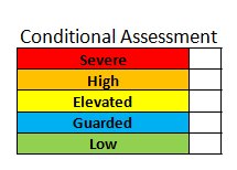
Sites are rated on a five-level conditional-assessment scale (Severe, High, Elevated, Guarded, Low) that feeds the probability × consequence matrix. Prioritized sites then receive one of four categories of risk control: drainage modifications, engineering, ground improvements or structural installations. Effectiveness is confirmed by follow-up geotechnical inspection over a minimum two-year evaluation period. The course gives approximate geotechnical monitoring budgets of $4–15M/year in the West, $2.5–4M/year in the East and $2.5–4M/year in the U.S., with capital spending up to $9M/year in the West.
Figures · click to zoom
After Geotechnology for Railroaders Program, Module 1; §10; slope stabilization process slides adapted from material by D. Colwell. Full reference under Supplemental Sources.
A rehabilitation plan has to justify the work as well as describe it. It should show a careful analysis of the existing track, bridges and facilities, tied to a clear statement of what the client needs the line to do. The same outline works for track, bridges and terminal facilities, and it fits the Plan phase of the stabilization program above.
| Section | Content | Benesch notes |
|---|---|---|
| 1. Operating requirements | Current and expected traffic: commodities, car types and numbers, train lengths, terminal and support facility needs | Use the traffic data checklist, Chapter 5, Table 5-S4 |
| 2. Description of track, bridges and facilities | Written description and condition, track maps and photographs. Give every track, bridge and turnout a unique designation. Station each track from 0+00 at the switch point where it leaves the main track; for a main track, start at the ownership limit or connection with the serving railroad | Stationing fixes work locations and quantities and gives permanent reference marks for later inspections; on mainline work, tie stations to mileposts (Chapter 5, §5.4) |
| 3. Deficiencies | Each major deficiency and how it keeps the facility from supporting the required operation; comparison with current design criteria; photographs | Draw on the condition, structural and operational evaluations |
| 4. Work plan | Remedial action and work limits for each deficiency, and why each action was chosen over the alternatives | If the plan doubles as contract documents, it must include full details of the work |
| 5. Cost estimate | Cost for each work-plan item | Major rehabilitation: cost the major items and add allowances for minor work. Single-stage plan: break the estimate down to contract level |
Points the work plan should address:
After UFC 4-860-01FA (2004), ch. 5, §6. Full reference under Supplemental Sources.
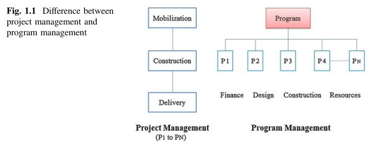
Haidar distinguishes program management, the coordinated delivery of a group of related projects, from managing each project on its own. A program passes through four stages: identification, planning, delivery and closure. Within it, the program manager handles pre-construction work (planning, site evaluation, cost and time parameters, bid packages), construction (contract award, procurement, cost and schedule monitoring, quality, safety, status reporting) and post-construction work (punch lists, open issues, warranty follow-up).
His program framework has four parts:
Program planning follows a fixed order: define objectives, agree the approach, agree roles, set communication channels, agree project priorities, then complete the project plans. At program level, each project becomes one activity in a higher-level network, and the planning is “macro”: cash flow, mobilization, crew allocation, heavy equipment distribution and delivery of critical materials. The benefits Haidar lists are a shared resource pool, less idle time, resource leveling across projects, knowledge carried from one project to the next, and reuse of equipment.
For railroad work: an annual grade and slope stabilization program, with dozens of sites across a division, fits this model directly. Treat each site as an activity in a program network, and plan the shared resources that actually limit delivery. These are track time on each subdivision, work trains and ballast or riprap supply, drill rigs and specialty contractors, flagging resources and the geotechnical staff who review designs. Sites on the same subdivision can be grouped so that one outage and one mobilization serve several repairs. The vision and benefits measures should be the railroad’s own, for example permanent slow orders removed or a lower ground-hazard incident rate on the treated segments. Closure includes handing over as-builts and monitoring records to the hazard inventory so that the next program year starts from current data.
Source: Haidar, A. D. (2016). Construction Program Management – Decision Making and Optimization Techniques. Cham, Switzerland: Springer International Publishing, pp. 2–13. Summarized and paraphrased; figures reproduced for internal reference. Full reference under Supplemental Sources.
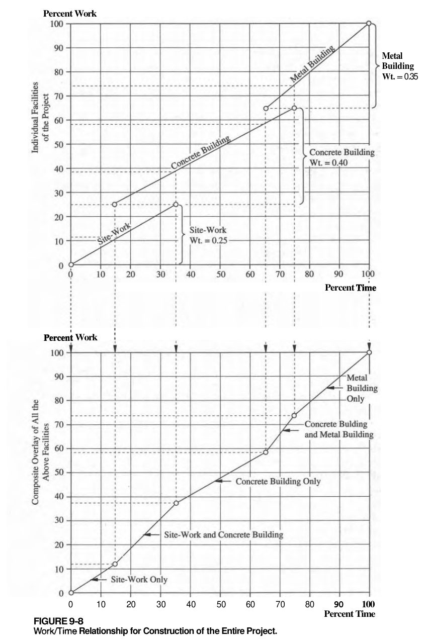
Oberlender warns that tracking only cost and time can mislead. A project may have spent half its budget at the schedule midpoint with only 20% of the work done; the cost and time curves look normal, and the overrun shows up too late to correct. His remedy is to measure work accomplished as a third variable, expressed as percent complete so that unlike units (cubic yards, pounds, drawings) can be combined.
Before work starts, the project manager and the people doing the work agree on weight multipliers that sum to 1.0, along with the expected timing of each task. His illustrative weights for design are shown below.
Table 1-PM1. Illustrative weight multipliers for design work (after Oberlender 2000, Table 9-5)
| Design task | Weight | Timing (% of duration) |
|---|---|---|
| Review backup material | 0.05 | 0–10 |
| Design calculations | 0.10 | 10–25 |
| Initial drafting | 0.25 | 15–45 |
| Final calculations | 0.20 | 35–60 |
| Production drawings | 0.30 | 50–90 |
| Drawing approval | 0.10 | 90–100 |
Superimposing the weighted tasks produces a planned work/time curve, which is plotted with the cost/time S-curve on a single integrated graph. Actual cost and actual work are then posted at each report date. His construction example shows why weighting matters: on a job with 18 drilled piers, all 18 have been drilled, steel is set in 9 and concrete placed in 3. Counting only cubic yards of concrete would show the piers 3/18 complete and ignore the drilling and steel already in place.
He adds that if a sponsor sets a milestone such as “60% design,” both parties must agree in advance on what 60% means.
For railroad work: A Grade & Slope Stabilization program carries many sites at once, each at a different stage. Assign each site weights that the program team agrees on at the start, for example investigation, analysis/concept, final design and GSPs, track-window construction, and post-construction monitoring. Program progress then becomes the budget-weighted sum across sites, not a count of sites “done.” Define the 30/60/90 review milestones in writing with the railroad’s engineering group. At the construction stage, weight sub-steps the same way (for example, for soldier piles: drilled, steel set, concreted, lagging placed) so that progress during short work windows is credited accurately.
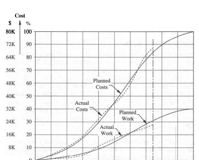
Source: Oberlender, G. D. (2000). Project Management for Engineering and Construction, 2nd ed. Boston: McGraw-Hill, pp. 134–138, 200–206. Summarized and paraphrased; figures reproduced for internal reference. Full reference under Supplemental Sources.
Levy (2007) outlines the components of a contractor safety program: a policy statement signed by top management; the objectives of the accident prevention program (planning work to minimize loss, prompt detection and correction of unsafe acts and conditions, enforced PPE and guarding, tool and equipment inspection, and training through orientation, periodic meetings and accident investigation); the duties of a safety director; the responsibilities of field supervisors, who are the first line of defense and run weekly toolbox talks; injury and illness reporting, with no discretion left to supervisors about what to report; working rules; a hazard communication program with safety data sheets on file; and a consistent progressive discipline policy.
He reproduces OSHA’s Construction Focused Inspection guideline, which checks for a designated competent person with authority to correct hazards and a project safety plan that includes a safety analysis at project start and at critical stages, identification of activities that need an engineer or competent person, procedures for hazardous operations such as cranes and trenching, documentation of inspections, hazard reports, incidents and near misses, and an emergency response plan. The four leading construction hazards cited are falls, struck-by, caught-in/between (including cave-ins) and electrical.
Levy also shows why safety matters financially. Workers’ compensation premium equals EMR × manual rate × payroll units (payroll ÷ 100). In his hypothetical example, the same $1.4 million payroll costs about $79,966 in total insurance with an EMR of 0.77 and premium credits, versus $187,859 at an EMR of 1.00, a difference of $107,893 in one year. Citing an insurer’s chart, he notes indirect accident costs are three to five times the insured cost, and that at a 2% profit margin $50,000 of new sales is needed to pay for a $1,000 accident.
For railroad work: A grade and slope stabilization program should require each contractor and drilling subcontractor to submit its safety program, EMR and recent OSHA history before award, and a site-specific plan that addresses roadway worker protection, excavation support next to track, and operation of equipment near live track. The plan’s project safety analysis should be repeated at critical stages, such as opening an excavation in the embankment toe or working during a track window.
Source: Levy, S. M. (2007). Project Management in Construction, 5th ed. New York: McGraw-Hill, pp. 300–315. Summarized and paraphrased. Full reference under Supplemental Sources.
Bissonette scores individual risks as probability rating × impact rating on a 5 × 5 matrix. In his example, scores of 10 or more are above tolerance and require a response, 4 or less go on a watch list, and those in between are decided case by case. He then adds three prioritization refinements that help when funds cannot cover every response:
He also uses a risk burn-down schedule, a plot of the summed severity scores over time that assumes the planned responses succeed. In his notional seven-month project, three risks initially total 40. Planned responses bring the total to 14 at the start of work, and it then steps down to 10, 8 and 5 as supplier, prototype and fabrication milestones pass, reaching 0 in month six. The baseline curve is compared with actual status to show when risk reduction is falling behind. He cautions that the absolute total is meaningful only within one project, not between projects.
For railroad work: In a grade and slope stabilization program, cost per severity point gives a defensible way to rank sites competing for one year’s budget. A low-cost ditch cleanout or horizontal drain that sharply lowers the probability score at one cut may outrank a costly wall at another site whose score falls by about the same amount. Timing matters as well. Investigation at sites where the remedy depends on unknown ground conditions should be scheduled early, so that the uncertainty is resolved before the work window. A program-level burn-down built from the planned completion dates of each site’s mitigation gives management a simple view of whether risk on the network is falling as planned.
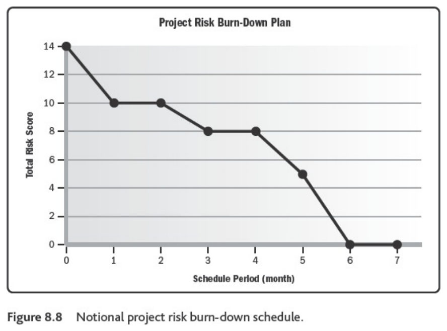
Source: Bissonette, M. M. (2016). Project Risk Management: A Practical Implementation Approach. Newtown Square, PA: Project Management Institute, Ch. 8 (unpaginated e-book; PDF pp. 105–118). Summarized and paraphrased; figures reproduced for internal reference. Full reference under Supplemental Sources.
Natural hazards are a significant, but not the predominant, cause of railway service disruption — in mountain territory they are actually less frequent than most other engineering-related incidents, accounting for on the order of 17% of engineering incidents by count. What makes them a distinct budget priority is that each incident carries a much higher average impact: roughly $1.5M per event in documented industry experience, working out to on the order of half of total engineering-incident cost despite the comparatively low incident count.
Because major geo-hazard occurrences fluctuate substantially year to year, the natural organizational tendency is to stay vigilant immediately after a significant event and then relax attention until the next one. A funded, followed R.M. plan is specifically designed to break that cycle — it forces sustained, proactive, yearly mitigation spending regardless of how recently an incident actually occurred. Because the consequence side of the risk equation is so high for natural-hazard scenarios, the same incident-cost data that justifies the program in the first place is also the strongest argument for securing its funding: a documented plan that is not consistently followed is worse, from both a safety and a liability standpoint, than having no plan at all.
Under European Regulation 1192/2003 a significant rail accident involves at least one rail vehicle in motion and results in at least one person killed or seriously injured, significant damage (at least €150,000) to rolling stock, track, other installations or the environment, or extensive interruption of traffic. In 2011 the 27 EU countries recorded 2,685 significant accidents, with 2,325 people killed or seriously injured. Of the fatalities, 60% were unauthorized persons, 29% level-crossing users, 5% passengers and 2% employees.
The causes listed by the book include inadequate track maintenance leading to derailment, mechanical failure of wheels and rails, an earthquake while a train is moving, and a collapsed bridge — the ground-hazard and track-support categories this manual addresses — alongside level crossings, signaling, switching and human factors. Accidents causing fatalities per billion train-km in the United Kingdom fell steadily from about 11 (1967–71) to below 1 (2007–10). For comparison, the book puts the risk of death at 7 times higher by car and 2 times higher by bus than by rail, and a route comparison for hazardous materials gave rail a risk factor about six times lower than road.
Figures · click to zoom
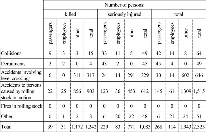
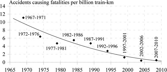
After Profillidis (2014), §22.6, Table 22.4, Fig. 22.17. Full reference under Supplemental Sources.
In mountain territory, natural hazards account for about 17% of engineering-related service incidents by count, but at roughly $1.5M per event they make up about 52% of engineering incident cost. The course also recommends spending about 3% of the operating budget on drainage and ditch maintenance. In practice that spending tends to lose out to rail and crossing work until poor drainage stops service.
Figures · click to zoom
After Geotechnology for Railroaders Program, Module 1; §01, §09. Full reference under Supplemental Sources.
Why the business case is hard to make. Selig and Waters note that substructure practice has been empirical. Trials take years to show results, maintenance and performance records are poor, and service demands keep changing. Technology spending is also the first thing cut because it shows no short-term return. A geotechnical recommendation therefore needs a cost argument as well as an engineering one.
Four points that support that argument.
After Selig & Waters (1994), chs. 1, 8, 15 and 16. Full reference under Supplemental Sources.
Rad treats cost, schedule and scope as linked. Changing any one moves the others.
Duration. Each activity has an optimum duration, the one that uses the optimum crew size and shift length and so has minimum cost. Departing from it costs more in either direction:
His crew example: one task takes 30 worker-days with 5 people over 6 days, 44 worker-days with 11 people over 4 days, and 60 worker-days with 20 people over 3 days. The losses come from congestion, extra communication and errors.
A schedule can be shortened in two ways:
He warns against padding the baseline with buffers to give away later. Once discovered, it ruins credibility.
Risk. For risk funding he describes a simple expected-value method. For each risk event, estimate the probability of occurrence and the cost if it occurs, and multiply them. The sum is the risk-related contingency. It can go into the project budget or into a separate earmarked fund, depending on how the project is financed.
For railroad work: Both ideas fit the business case for ground-hazard mitigation. For the expected-value calculation, an illustrative register might include:
These give a defensible contingency line. The project-specific numbers must come from the investigation and the railroad’s own incident records.
For schedule compression, track-window and possession limits often force remediation work into compressed durations. The extra crews, equipment standby and lower productivity that follow should be priced explicitly, not assumed free. When comparing a short-window intensive program with a longer program under a slow order, include the slow-order delay costs and the compression premium in the same comparison.
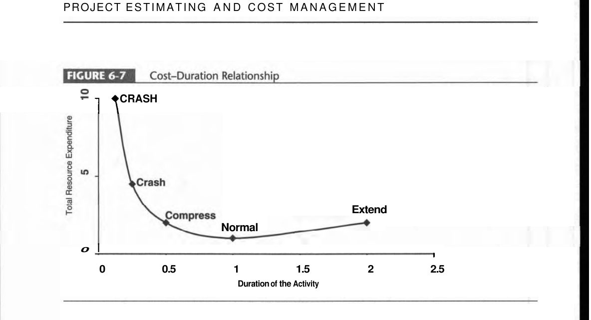
Source: Rad, P. F. (2002). Project Estimating and Cost Management. Vienna, VA: Management Concepts, pp. 88–96. Summarized and paraphrased; figures reproduced for internal reference. Full reference under Supplemental Sources.
Sullivan et al. define the conventional B–C ratio as:
B–C = PW(benefits) / [initial investment − PW(salvage) + PW(O&M)]
The modified ratio instead subtracts O&M from the numerator. The two give different numbers but always the same accept/reject decision, as long as the ratio is tested against 1.0. The same holds whether disbenefits are subtracted from benefits or added to costs, and whether a maintenance saving is counted as a benefit or as a reduced cost.
The trap is choosing among mutually exclusive alternatives by the highest ratio. The correct procedure (Figure 10-3) has four steps:
In their Example 10-7 at 10% over 50 years, Project A has B–C = 1.34. The B−A increment fails (0.91), but the C−A increment passes (1.16), so C is selected. A has the highest ratio of the three, yet it is not the right choice.
Their case study on a railroad grade-crossing overpass shows why the evaluator’s point of view matters. The city counts the delay to the 2,000 vehicles a day held at the crossing, plus avoided accident costs: about $257,000/yr in benefits against $88,500/yr in annualized costs, for B–C = 2.91. The railroad’s own $30,000/yr saving on crossing protection and claims is left out of the city’s ratio. That saving is worth about $199,000 to the railroad at its 15% cost of capital over 40 years, which gives a sound basis for asking the railroad to contribute.
For railroad work: for a chronic slope or subgrade problem, list the mutually exclusive alternatives:
For each alternative, count as benefits the avoided train-delay cost of the slow order, the avoided maintenance, and the reduction in expected incident losses. Run the incremental test rather than ranking by ratio. Where public grant funding is involved, show the analysis from both the public and the railroad point of view, with the discount rate each one uses.
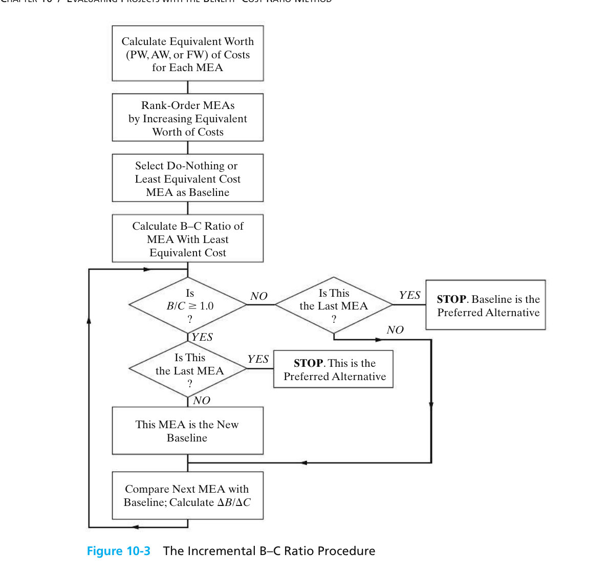
Source: Sullivan, W. G., Wicks, E. M. and Koelling, C. P. (2015). Engineering Economy, 16th ed. Upper Saddle River, NJ: Pearson, pp. 449–467. Summarized and paraphrased; figures reproduced for internal reference. Full reference under Supplemental Sources.
The CIOB Code treats the last stage of a project as more than paying the final invoice. Its outcomes include settling claims, finalizing payments, archiving records, recording residual risks, and a post-project review that answers one question: has the project satisfied the need? The Code organizes the review into several parts:
For railroad work: For a ground hazard program, the “benefits realization” question is concrete: after the repair, did the site stop generating slow orders, track geometry defects, maintenance tamping or incident reports? Make a short close-out report a standard deliverable for each Grade & Slope Stabilization site. It should cover:
Feeding these results back into the risk ranking and unit-cost history is what lets the business case in Section 1.11 rest on the program’s own performance data rather than assumptions.
Source: Chartered Institute of Building (2014). Code of Practice for Project Management for Construction and Development, 5th ed. Chichester, UK: John Wiley & Sons, pp. 307–310. Summarized and paraphrased. Full reference under Supplemental Sources.
Q1. A field engineer finds a section of embankment where a blocked culvert has forced ditch water through the fill, producing visible seepage and minor slumping at the toe, directly beneath a passenger-service main line. Using the risk equation, explain why this scenario may warrant an “unacceptable” risk classification even if the hazard itself (seepage-induced slumping) would rate only Elevated in isolation.
A: Risk = Hazard × Consequence & Vulnerability. The hazard rating alone (Elevated) does not capture the consequence side: an embankment failure beneath active passenger service carries a catastrophic potential outcome (derailment with injury/fatality exposure), which the risk equation multiplies against the hazard rating rather than averaging with it. In UNDRR terms, the passenger trains are the exposure and the saturated embankment above the drop is the vulnerability; both are high, so the risk is high even though the hazard is not. Per the risk resolution matrix (§17.7), even an “Occasional” probability crossed with a “Catastrophic” consequence still resolves to Unacceptable, meaning immediate risk control (speed restriction, inspection, or culvert repair) is warranted regardless of how the hazard alone would be scored.
Q2. Classify the following observed condition using the three-category system in §17.3, and identify whether it is progressive or sudden-onset: a section of yard track has developed a gradual, several-inch-per-year settlement over a former peat bog, with no sudden void collapse observed to date.
A: This is a subsidence hazard (not landslide or hydraulic erosion, since there is no slope-movement or erosion mechanism described), specifically progressive settlement (consolidation/muskeg-type behavior) as opposed to sudden collapse. Per §17.6, the typical risk rating for this hazard type is Elevated, and the standard diagnostic step before selecting a repair (excavation/geotextile trench, French drain, or cement powder fill) is confirming the actual mechanism — since a visually identical “muddy track” symptom can also result from ballast mud-spot failure or a failing culvert, which call for different fixes.
| Related Topic | Chapter |
|---|---|
| Groundwater characterization, seepage, and piezometer monitoring behind hydraulic-erosion and subsidence hazards | Chapter 9 |
| Slope stability analysis and factor-of-safety methods underlying landslide risk scoring | Chapter 13 |
| Seismic hazard and liquefaction assessment referenced by earthquake notification response | Chapter 14 |
| Ground improvement methods used as risk-control measures once a site enters mitigation | Section 17.16 (17.16.1–17.16.45) |
| Retaining structures as a structural risk-control option | See the Retaining Structures chapter (Chapter 16) |
| Railroad track subgrade failure modes referenced under subsidence hazards | Chapter 2 |
| Construction monitoring and instrumentation used during stabilization effectiveness review | Chapter 15 |
| Geotechnical report preparation and documentation of risk-management decisions | Appendix E |
Chapter 1 — Introduction to Railway Ground Hazard Risk Management
Primary Source: Geotechnology for Railroaders Program, Module 1; Keegan, Abbott & Ruel (2004), A Risk Management Framework for Ground Hazards Along Canadian National Railways; CAN/CSA-Q850-97.
Field case studies by Burt G. Look, from Earthworks: Theory to Practice – Design and Construction (CRC Press/Balkema, 2023), chosen for this chapter’s topics. Each is summarized from the book with its key figures and a closing note on railroad application added by the authors of this manual. Credit for the case material belongs to Look; see item S13 under Supplemental Sources.
Related section: 1.5 Hydraulic Erosion Hazards
Look (1999) back-analysed a riverbank failure on the Brisbane River at St Lucia, in front of a boat shed. Soil variability was combined with tidal water levels, using known mean high and low water spring levels as the time factor for groundwater. The adjacent stable bank had an annual probability of failure of about 10−3 at operating water levels. At the slide itself the calculated probability was 14%, and along the “stable” length of the boat shed it was 7.5%.
The first advice was to move the boat shed, but the owner considered it important enough to keep. Repairs cost 2.5 times the structure at risk. The 7.5% figure justified extending the works along the whole shed: two rows of timber piles at the failure, one row along the rest.
Four activating factors combined: vegetation removed a few weeks earlier; topsoil and a concrete path placed at the crest; an unusual tide on the day; and a new boat service that had started a few weeks before. Deep-seated failures like this are costly but rare. Shallow failures are far more common and call for regular inspection and maintenance before they grow.
For railroad work: where track runs along a river, back-analysis of a failed reach can set the extent of the repair along the “stable” bank next to it. Vegetation clearing, fill at the crest and new wave sources such as boat traffic or channel work are triggers to log in the hazard inventory.
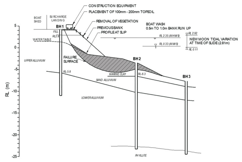
Source: Look, B. G. (2023). Earthworks: Theory to Practice – Design and Construction. CRC Press/Balkema. Case study §9.8, pp. 304. Summarized and paraphrased; figures reproduced for internal reference. Full reference under Supplemental Sources.
Related section: 1.7 Risk Scenarios and Risk Estimation
Brisbane’s 2010/11 summer brought 37.5 in of rain against a 16.3 in average. Rockfalls from urban road cuts, road failures at cross-drainage, fill failures at creek banks and extensive slides along the Brisbane River followed. The emergency phase lasted three months, with repairs continuing for years. Look draws out several points for landslide risk management:
His examples run from a blocked drain on a gated private road (insignificant) through a local road with diverted traffic and load limits (low to medium) to a slip on a blind curve, caused by undersized culverts sending water across the road, where barriers and signals cut a major consequence to minor.
For railroad work: in a ground hazard risk estimate (§1.7), the consequence term should include remediation and reinstatement cost, service interruption and detour feasibility, not only the value of what is damaged. Immediate controls such as slow orders, patrols and protective barriers move a site down the consequence scale while the permanent fix is designed.
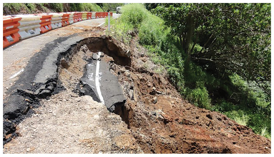
Source: Look, B. G. (2023). Earthworks: Theory to Practice – Design and Construction. CRC Press/Balkema. Case study §9.3.3, pp. 280–284. Summarized and paraphrased; figures reproduced for internal reference. Full reference under Supplemental Sources.
Related section: 1.8 Purpose-Built Assessment Tools
Look sets four scales of slope assessment side by side: limit equilibrium (deterministic or probabilistic site study), finite element with strength reduction, monitoring (an observational, site-specific approach), and GIS hazard weighting for regional planning. Look (2005) describes a GIS study for a fast-growing Shire in Queensland, commissioned for planning, with no significant landslips on record and little landslide data.
Weighting factors were applied to lithology and structure, slope morphometry, relative relief, slope aspect, land cover and environmental factors. Risk was assessed by laying existing and proposed development over the hazard map, with extra attention to travel distance and to areas near waterways that are prone to slips in floods. Practical points:
For railroad work: network-scale ground hazard screening is the same problem with a linear asset. Calibrate the weightings against the railroad’s own incident and slow-order history, and treat the output as a list of where to look, not a risk rating.
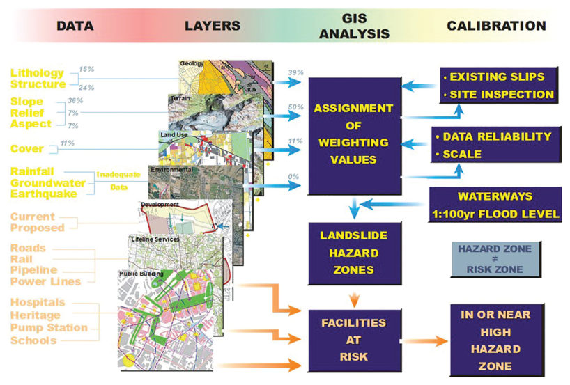
Source: Look, B. G. (2023). Earthworks: Theory to Practice – Design and Construction. CRC Press/Balkema. Case study §9.9, pp. 304–308. Summarized and paraphrased; figures reproduced for internal reference. Full reference under Supplemental Sources.
Authors: Daniel P. Colwell and Mario Ruel. This chapter was written and compiled by Daniel P. Colwell and Mario Ruel for Railway Ground Hazard Risk Management.
Technical content is drawn from the published sources below, and credit for that material belongs to their authors and publishers. Tables, equations and figures taken from a specific source are also cited where they appear.
File locations for these documents are listed under Supplemental Sources — LEVI Library.
Material in the green “Supplemental reference” boxes throughout this chapter was added from the following documents in the LEVI geotechnical library. Text is summarized or paraphrased; tables are reproduced with their original source noted; figures are reproduced from the cited document for internal reference use. Consult the original document before relying on a value for design. Blocks marked “After UFC 4-860-01FA (2004)” draw on item S11 and are rewritten for railroad clients. Blocks marked “After Selig & Waters (1994)” summarize item S12 for railroad clients; tables are condensed from the book and its figures are not reproduced. The Case Studies section summarizes case studies from item S13 by Burt G. Look; its figures are reproduced from the book for internal reference use, and the closing “For railroad work” note in each case study is added by the authors of this manual. Blocks tagged “Project management” summarize methods, examples and figures from the project-management, estimating and construction-management books listed here, applied to railroad work; the closing “For railroad work” note in each block is added by the authors of this manual.